Building Essential in 4 Dimensions

Version 1.00

U Win Aung Cho

B.E. Civil.

M.Civ.Eng.

Blk. No.6/ Room 002

Station Road Aye-yeik-Mon

Estate (1)

Hlaing Township

19-May-2006

Sample Screen Shots of BE4D Application.

At Z direction grid level, columns will be seen and grid label, line and dimension of grid spacing are also included.

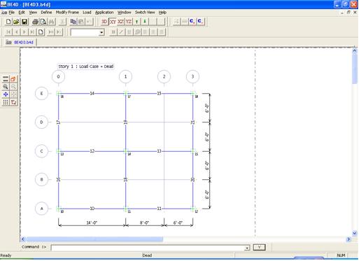
Figure 1 Plan View

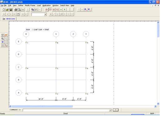
Figure 2 Plan View at Base

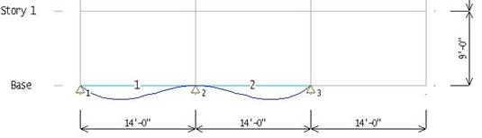
Columns and Beams are differently visible with color and grid label, line and dimension of grid spacing are also shown.

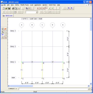
Figure 3 Elevation View at 1

Figure 4 Elevation View at A

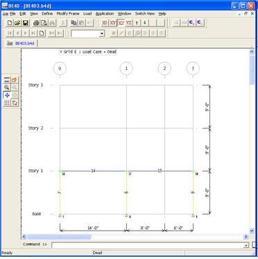
Figure 5 Elevation View at E

Isometric views and Perspective views are implemented. View point and camera position can be arbitrarily changed.

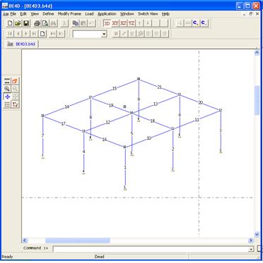
Figure 6 Iso-View

Input data and output data can be seen in table view. Table can be copied onto clip-board and copied data can be pasted on common applications such as notepad, M.S. word and excel.

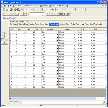
Figure 7 Table View for Member Detail

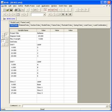
Figure 8 Table View for Grid

Nice dialog design enhances to ease data input.

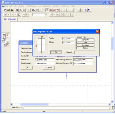
Figure 9 Dialog Sample for Section

Selected elements (nodes and frames) can be repeatedly modified to meet user needs and several trials are allowed unlimitedly.

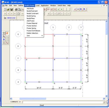
Figure 10 Menu for Member Assignments

Programming facility

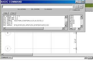
Built-in BASIC interpreter supplies numerous commands and functions for model creation and modification.

Sample Program

10 addnode 0,0

20 addnode 14,0

30 addnode 28,0

40 addres 1 1 2 3

50 addres 2 1 2 3

60 addres 3 1 2 3

130 addframe 1,2

140 addframe 2,3

150 addmat 3122*144,1500*144,0.15,0.15/32.2

160 b=0.75

170 d=0.75

180 addsec b*d,b*d^3/12,d*b^3/12,b*d*(b^2+d^2)/12

Printing facility

All views can be printed as you see and project information is allowed at header and footer places. Project information can be changed in sheet settings.

Text file Support

Input and Output data may be in simple ASCII text file. Input text file is importable and editable in BE4D Text View.

Text Output Sample

Log Information

After running analysis program, it send log information to command window as follow.

Start RunAnalysis

Start printKnM

printing stiffness and mass for data NoName

Start FormKnM

Forming stiffness and mass

allocated size of stiffness matrix (bytes) = 576l

allocated size of mass matrix (bytes) = 576l

forming stiffness matrix of element... 1

.... placing in global locations

Finished Stiffness and Mass

End FormKnM

num. of dof bandwidth

12 12

printing banded stiffness matrix

printing banded mass matrix

printing starting vector for inverse iteration

finished stiffness and mass for data NoName

End printKnM

Start Geneigen

Generating eigen value & eigen vector

Start Invitr

no convergence for 101 iterations of 4

End Invitr

Finished Generating 3 eigen values & eigen vectors

End Geneigen

Start LoadK

reading stiffness data

stiffness and mass for data NoName num. of dof bandwidth

num. of dof bandwidth

12 12

allocated size of stiffness matrix (bytes) = 576l

finished loading

End LoadK

Start solver

Start Solving

Finished Solving

End solver

Start LoadK

reading stiffness data

stiffness and mass for data NoName num. of dof bandwidth

num. of dof bandwidth

12 12

allocated size of stiffness matrix (bytes) = 576l

finished loading

End LoadK

Start solver

Start Solving

Finished Solving

End solver

Result are in Files C:\DOCUME~1\UWINAU~1\LOCALS~1\Temp\NoName.txt & C:\DOCUME~1\UWINAU~1\LOCALS~1\Temp\NoName.eig

End RunAnalysis

Frame Information

Typing a command FRAMEINFO in command prompt, program send following output summary in command window in text format.

FRAMEINFO

Start NodalData

1 +0.000E+000 +0.000E+000 +0.000E+000

+0.000E+000 +0.000E+000 +0.000E+000 +0.000E+000 +0.000E+000 +0.000E+000

2 +1.000E+001 +0.000E+000 +0.000E+000

+0.000E+000 +0.000E+000 +0.000E+000 +0.000E+000 +0.000E+000 +0.000E+000

Reference Node

End NodalData

Start ElementData

1 1 2 0 1 1

+0.00E+000 +0.00E+000 +0.00E+000

End ElementData

Start MaterialData

1 Concrete 4.104E+005 1.710E+005 1.500E-001 4.658E-003 5.500E-006

End MaterialData

Start SectionData

1 B9x12 7.500E-001 3.516E-002 6.250E-002 7.593E-002 9.375E-002 1.250E-001 2.165E-001 2.887E-001

2 1.000E+000 8.333E-002 8.333E-002 1.408E-001 0.000E+000 0.000E+000 0.000E+000 0.000E+000

3 0.000E+000 0.000E+000 0.000E+000 0.000E+000 0.000E+000 0.000E+000 0.000E+000 0.000E+000

End SectionData

Start RestraintData

1 ux 0.0000e+000

1 uy 0.0000e+000

1 uz 0.0000e+000

1 rx 0.0000e+000

1 ry 0.0000e+000

1 rz 0.0000e+000

End RestraintData

Start ConstraintData

End ConstraintData

Start SpringData

End SpringData

Start LoadData

1 Dead 0 1.000E+000

Nodal Load

1 +0.000E+000 +0.000E+000 +0.000E+000 +0.000E+000 +0.000E+000 +0.000E+000

2 +0.000E+000 +0.000E+000 +0.000E+000 +0.000E+000 +0.000E+000 +0.000E+000

Element Load

1 +0.00E+000 +0.00E+000 +0.00E+000

2 Live 1 0.000E+000

Nodal Load

1 +0.000E+000 +0.000E+000 +0.000E+000 +0.000E+000 +0.000E+000 +0.000E+000

2 +0.000E+000 +0.000E+000 +0.000E+000 +0.000E+000 +0.000E+000 +0.000E+000

Element Load

1 +0.00E+000 +0.00E+000 +0.00E+000

End LoadData

Start NodalDisplacement

Dead

node# ux uy uz rx ry rz

1 +0.000e+000 +0.000e+000 -3.6550e-013 +0.000e+000 +1.827e-012 +0.0000e+000

2 +0.000e+000 +0.000e+000 -5.4825e-003 +0.000e+000 +7.310e-004 +0.0000e+000

Live

node# ux uy uz rx ry rz

1 +0.000e+000 +0.000e+000 +0.0000e+000 +0.000e+000 +0.000e+000 +0.0000e+000

2 +0.000e+000 +0.000e+000 +0.0000e+000 +0.000e+000 +0.000e+000 +0.0000e+000

End NodalDisplacement

Start Reaction

Dead

1 Fx +0.0000e+000

1 Fy +0.0000e+000

1 Fz +1.1250e+000

1 Mx +0.0000e+000

1 My -5.6250e+000

1 Mz +0.0000e+000

Live

1 Fx +0.0000e+000

1 Fy +0.0000e+000

1 Fz +0.0000e+000

1 Mx +0.0000e+000

1 My +0.0000e+000

1 Mz +0.0000e+000

End Reaction

Start Spring_action

Dead

Live

End Spring_action

Start ElementForces

member end-forces

Dead

member # 1

+0.0000e+000 +1.1250e+000 +0.0000e+000 +0.0000e+000 +0.0000e+000 +5.6250e+000

+0.0000e+000 +8.3819e-009 +0.0000e+000 +0.0000e+000 +0.0000e+000 -5.5879e-008

Live

member # 1

+0.0000e+000 +5.6250e-001 +0.0000e+000 +0.0000e+000 +0.0000e+000 +9.3750e-001

+0.0000e+000 +5.6250e-001 +0.0000e+000 +0.0000e+000 +0.0000e+000 -9.3750e-001

End ElementForces

Start ModalResult

Start NormalizeModeVector

End NormalizeModeVector

Inverse Iteration Method for Eigenvalues and Eigenvectors

Number of Modes desired 12

Number of Modes found 3

Mode number 1 Natural Period T = 1.262e-001 sec

Circular Freq. = 4.978e+001 rad/sec Natural Freq. = 7.922e+000 hz

Eigenvector

node# ux uy uz rx ry rz

1 +0.000e+000 +1.406e-011 +1.411e-014 +0.000e+000 -1.411e-013 +1.406e-010

2 +8.410e-038 +1.000e+000 +5.644e-004 +0.000e+000 -8.466e-005 +1.500e-001

Mode number 2 Natural Period T = 9.467e-002 sec

Circular Freq. = 6.637e+001 rad/sec Natural Freq. = 1.056e+001 hz

Eigenvector

node# ux uy uz rx ry rz

1 +1.559e-016 -1.411e-014 +2.500e-011 +0.000e+000 -2.500e-010 -1.411e-013

2 +1.559e-008 -1.003e-003 +1.000e+000 +0.000e+000 -1.500e-001 -1.505e-004

Mode number 3 Natural Period T = 4.733e-003 sec

Circular Freq. = 1.327e+003 rad/sec Natural Freq. = 2.113e+002 hz

Eigenvector

node# ux uy uz rx ry rz

1 +1.000e-008 +2.546e-016 -1.949e-015 +0.000e+000 +1.949e-014 +2.546e-015

2 +1.000e+000 +1.810e-005 -7.795e-005 +0.000e+000 +1.169e-005 +2.716e-006

End ModalResult

Auto Load Calculation

Self Weight

Self-weight can be included in any static load case by increasing self weight multiplyer.

Auto Seismic Load

Program support Auto Seismic Load according to UBC 97. Minimum equivalent lateral load is applied on each node according to their mass lumped at node.

Response Spectrum Analysis

After modal analysis (Eigen Method), It calculate response spectrum analysis as mention in UBC 97 Code.

Analysis Types

Software is capable to solve following analysis.

1) Static Linear Analysis

2) Modal Analysis (Free-Vibration)

3) Response Spectrum Analysis